INTRODUCTION TO MATLAB

1.5 Pause command
A pause command in a script causes execution to stop temporarily. To continue just hit
Enter. You can also give it a time argument like this

pause(.2)

which will cause the script to pause for 0.2 seconds, then continue. And, of course, you can
ask for a pause of any number or fractions of seconds. Note, however, that if you choose
a really short pause, like 0.001 seconds, the pause will not be so quick. Its length will be
determined instead by how fast the computer can run your script.

1.6 Online Help
If you need to find out about something in Matlab you can use help or lookfor at the
>>prompt. There is also a wealth of information under Help Desk in the Help menu
of Matlab's command window. For example maybe you are wondering about the atan2
function mentioned in Sec. 1.2. Type

help atan2

at the >>prompt to find information about how this form of the inverse tangent function
works. Also type

help bessel

to find out what Matlab's Bessel function routines are called. Help will only work if you
know exactly how Matlab spells the topic you are looking for.

Lookfor is more general. Suppose you wanted to know how Matlab handles elliptic
integrals. help elliptic is no help, but typing

lookfor elliptic

will tell you that you should use

help ellipke

to find what you want.

1.7 Making Matlab Be Quiet
Any line in a script that ends with a semicolon will execute without printing to the screen.
Try, for example, these two lines of code in a script or at the >> command prompt.

a=sin(5),
b=cos(5)

Even though the variable a didn't print, it is loaded with sin (5), as you can see by typing
this:

a

1.8 Debugging
When your script fails you will need to look at the data it is working with to see what went
wrong. In Matlab this is easy because after you run a script all of the data in that script
is available at the Matlab >>prompt. So if you need to know the value of a in your script
just type

a

and its value will appear on the screen. You can also make plots of your data in the
command window. For example, if you have arrays x and y in your script and you want to
see what y(x) looks like, just type plot(x,y) at the command prompt.

The following Matlab commands are also useful for debugging:

who lists active variables
whos lists active variables and their sizes
what lists .m files available in the current directory

This information is also available in the workspace window on your screen and described in
the next section.

1.9 Arranging the Desktop
A former student, Lance Locey, went directly from this Introduction to Matlab to doing
research with it and has found the following way of arranging a few of Matlab's windows on
the desktop to be very helpful. (A visual representation of this layout appears in Fig. 1.1.)

1. Make the command window wide and not very tall, stretching across the bottom of
the desktop.
2. Open a script editing window (click on the open-a- le icon on the tool bar) and place
on the left side, just above the command window.
3. Click on View on the tool bar, then on Workspace to open the workspace window,
and place it at the upper right.

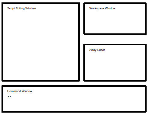
Figure 1.1 A convenient arrangement of the desktop

4. In the command window type a=1 so that you have a variable in the workspace
window, then double click on the yellow name icon for a in the workspace window
to make the Array Editor appear. Then place this window just below the workspace
window and above the command window, at the left side of the desktop (see the next
page.)

With these windows in place you can simultaneously edit your script, watch it run in the
command window, and view the values of variables in the array editor. You will find that
this is very helpful later when our scripts become more complicated, because the key to
debugging is to be able to see the sizes of the arrays that your script is using and the
numerical values that they contain. In the next section you will work through a simple
example of this procedure.

1.10 Sample Script
To help you see what a script looks like and how to run and debug it, here is a simple one
that asks for a small step-size h along the x-axis, then plots the function cos x
from x = 0 to x = 20. The script then prints the step-size h and tells you that it is finished.
The syntax and the commands used in this script are unfamiliar to you now, but you will
learn all about them shortly. Type this script into an M- le called test.m using Matlab's
editor with the desktop arranged as shown on the previous page. Save it, then run it by
typing

test

in the command window. Or, alternatively, press F5 while the editing window is active and
the script will be saved, then executed. Run the sample script below three times using these
values of h: 1, 0.1, 0.01. As you run it look at the values of the variables h, x, and f in the
workspace window at the upper right of the desktop, and also examine a few values in the
array editor just below it so that you understand what the array editor does.

1.11 Breakpoints and Stepping
When a script doesn't work properly, you need to find out why and then x it. It is very
helpful in this debugging process to watch what the script does as it runs, and to help you
do this Matlab comes with two important features: breakpoints and stepping.

To see what a breakpoint does, put the cursor on the x=0:h:20 line in the sample script
above and either click on Breakpoints on the tool bar and select Set/Clear, or press F12.
Now press F12 repeatedly and note that the little red dot at the beginning of the line toggles
on and o , meaning that F12 is just an on-o switch set set a breakpoint. When the red
dot is there it means that a breakpoint has been set, which means that when the script
runs it will execute the instructions in the script until it reaches the breakpoint, and then
it will stop. Make this happen by pressing F5 and watching the green arrow appear on the
line with the breakpoint. Look at the workspace window and note that h has been given a
value, but that x has not. This is because the breakpoint stops execution just before the
line on which it is set.

Now you can click on the Debug icon on the tool bar to see what to do next, but the
most common things to do are to either step through the code executing each line in turn
(F10) while watching what happens to your variables in the workspace and array editor
windows, or to just continue after the breakpoint to the end (F5.) Take a minute now and
use F10 to step through the script while watching what happens in the other windows.

When you write a script to solve some new problem, you should always step through it
this way so that you are sure that it is doing what you designed it to do. You will have lots
of chances to practice debugging this way as you work through the examples in this book.

Chapter 2
Variables

Symbolic packages like Mathematica and Maple have over 100 different data types, Matlab
has just three: the matrix, the string, and the cell array. In both languages variables are
not declared, but are defined on the y as it executes. Note that variable names in Matlab
are case sensitive, so watch your capitalization. Also: please don't follow the ridiculous
trend of making your code more readable by using long variable names with mixed lowerand
upper-case letters and underscores sprinkled throughout. Newton's law of gravitation
written in this style would be coded this way:

Force_of_1_on_2 = G*Mass_of_1*Mass_of_2/Distance_between_1_and_2^2

You are asking for an early end to your programming career via repetitive-stress injury if
you code like this. Do it this way:

F=G*m1*m2/r12^2

2.1 Numerical Accuracy
All numbers in Matlab have 15 digits of accuracy. When you display numbers to the screen,
like this
355/113

you may think Matlab only works to 5 significant figures. This is not true, it's just displaying
five. If you want to see them all type
format long e

The four most useful formats to set are
format short (the default)
format long
format long e
format short e

Note: e stands for exponential notation.

2.2 π

Matlab knows the number π.
pi

Try displaying π under the control of each of the three formats given in the previous section.
Note: you can set pi to anything you want, like this, pi=2, but please don't.

2.3 Assigning Values to Variables
The assignment command in Matlab is simply the equal sign. For instance,
a=20

assigns 20 to the variable a.

2.4 Matrices
Matlab thinks the number 2 is a 1x1 matrix:
N=2
size(N)

The array
a=[1,2,3,4]
size(a)

is a 1x4 matrix (row vectors are built with commas), the array
b=[1;2;3;4] size(b)

is a 4x1 matrix (column vectors are built with semicolons, or by putting rows on separate
lines-see below.)
The matrix
c=[1,2,3,4,5,6;7,8,9]
size(c)

is a 3x3 matrix (row entries separated by commas, different rows separated by semicolons.)
It should come as no surprise that the Mat in Matlab stands for matrix.

When matrices become large the , and , way of entering them is awkward. A more
visual way to type large matrices in a script is to use spaces in place of the commas and to
press the Enter key at the end of each row in place of the semicolons, like this:

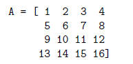
This makes the matrix look so nice in a script that you probably ought to use it exclusively.

When you want to access the elements of a matrix you use the syntax A(row,column).
For example, to get the element of A in the 3rd row, 5th column you would use A(3,5).
And if you have a matrix or an array and you want to access the last element in a row or
column, you can use Matlab's end command, like this:
c(end)
A(3,end)

2.5 Strings
A string is a set of characters, like this
s='This is a string'

And if you need an apostrophe in your string, repeat a single quote, like this:
t='Don''t worry'

And if you just want to access part of a string, like the first 7 characters of s (defined above)
use
s(1:7)

Some Matlab commands require options to be selected or set by using strings. Make
sure you enclose them in single quotes, as shown above. If you want to know more about
how to handle strings type help strings.