Linear Algebra Notes

1 Algebra of Matrices

1.1 Definition

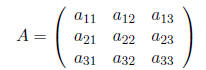
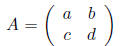
Definition 1 A m × n matrix A is a table with m rows and n columns written:

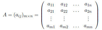
where the (ij)^th element of A is

Definition 2 Two matrices A and B are said to be equal (A = B) if and only if they have the
same number of rows and columns m × n, and

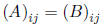
for all i = 1, . . . ,m and j = 1, . . . , n.

1.2 Addition

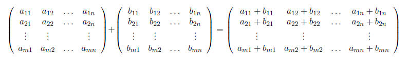
Definition 3 Matrix addition: If or

Theorem 1 If A, B, C are m × n matrices, then

A + B = B + A

and

(A + B) + C = A + (B + C)

Definition 4 The zero matrix (0)_m×n is the m × n matrix where each entry is 0. When the size
of the matrix is understood, the zero matrix is sometimes simply written as 0.

1.3 Scalar multiplication

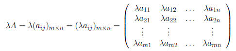
Definition 5 Scalar multiplication: If λ is a scalar and A a m × n matrix, then

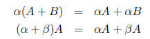
Theorem 2 If are scalars and A,B are m × n matrices, then

1.4 Matrix multiplication

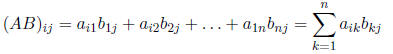
Definition 6 Matrix multiplication: If then the product AB is a
m × p matrix where

Remark 1 In general, AB ≠ BA.

Remark 2 If A is an m × n matrix, then

Remark 3 It is possible for AB = 0 with A ≠ 0 and B ≠ 0.

Theorem 3 A(BC) = (AB)C

Theorem 4 A(B + C) = AB + AC and (B + C)A = BA + CA.

Theorem 5 If λ is a scalar and AB is defined, then λ(AB) = (λA)B = A(λB).

Definition 7 The n × n matrix I or I_n×n defined by

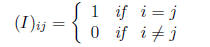
is called the identity matrix.

Theorem 6 AI = IA = A.

Definition 8 A matrix D is called diagonal if it is a scalar multiple of the indentity matrix:

Definition 9 If AB = BA then A and B are said to commute.

1.5 Transpose

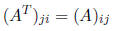
Definition 10 If A is a m×n matrix, the transpose of A, written A^T or A' is the n×m matrix
where

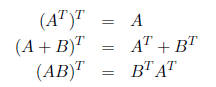
Theorem 7 The following properties hold for matrix transpose operations, where A and B are
matrices of appropriate dimensions:

Definition 11 A matrix A is symmetric if A = A^T , and skew-symmetric if A = −A^T .

Remark 4 If A is a square matrix, then the matrix A+A^T is symmetric, and the matrix A−A^T
is skew-symmetric.

1.6 Inverse

Definition 12 The inverse of the square matrix A is a matrix A^-1 such that

If A has an inverse, it is said to be invertible.

Remark 5 Not all square matrices are invertible.
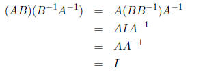
Remark 6 If A and B are invertible, then

since

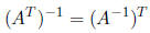
Remark 7 If A is invertible, then

Definition 13 A square matrix A is called orthogonal if A^-1 = A^T .

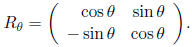
Definition 14 The rotation matrix

Remark 8 If (x, y) represent coordinates of a point or vector in the plane, then

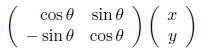
rotates (x, y) by θ.

Remark 9 The rotation matrix R_θ is orthogonal.

2 Vector Spaces

2.1

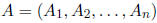
Definition 15 The vector space is the set of ordered n-tuples of real numbers ,
where addition is defined by

and scalar multiplication is defined by

with the zero element 0 = (0, . . . , 0).

Remark 10 The vector space can be also represented as the set of n × 1 matrices (column
vectors)

or 1 × n matrices (row vectors)

where are real numbers.

For example, the vector space R² is the set of ordered pairs (x, y) where x, y are real numbers.
Geometrically, this represents the xy-plane. The vector space R³ is then the 3-dimensional space
of real numbers (x, y, z), etc.

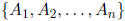
Definition 16 A set of vectors in the vector space are linearly independent if
the only way for the equation

to hold is if the scalars Otherwise, the set of vectors is called linearly
dependent.

In R², the set {(1, 0), (0, 1)} is linearly independent, while the sets {(1, 2), (3, 6)} and {(1, 0), (0, 1), (0, 2)}
are linearly dependent.

Definition 17 The dimension of a set of vectors is the maximum number of linear
independent vectors in the set.

2.2 Linear transformations

Definition 18 A linear transformation T from the vector space

is a linear function from

Remark 11 A m × n matrix is an example of a linear transformation from the vector space
: the matrix takes column vectors from and gives back a vector in . We can think of
a m × n matrix as n column vectors of length m stacked side by side.

Definition 19 The kernel or null space of a linear transformation , written ker(T),
is the set of all vectors in Rm such that

Definition 20 The rank of a m×n matrix , where each is a m×1 column
vector, is the dimension of its set of column vectors .

3 The Determinant

3.1 Definition

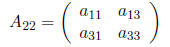
Consider the m×n matrix A and define the (m−1)×(n−1) submatrix as the matrix obtained
from A by deleting the ith row and jth column. For example, if

then the submatrix is obtained by deleting the second row and second column:

We will define the determinant of a matrix recursively, by first defining the determinant of a number

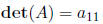
Definition 21 The determinant of a 1 × 1 matrix A = (a₁₁) is

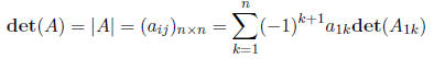
Definition 22 The determinant of a n × n matrix A is

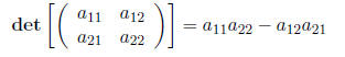
Using this, we can write down the determinant of a 2 × 2 matrix as

and a 3 × 3 matrix as

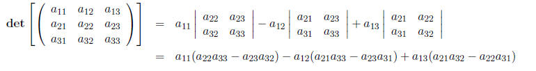
Note that so far we are expanding the determinants along the first row. The general definition of
the determinant, however, allows us to expand along any row or column.

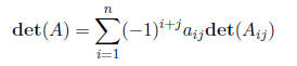
Definition 23 For any fixed row index i, the determinant of a n × n matrix A is

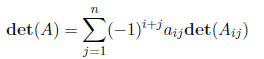
Definition 24 For any fixed column index j, the determinant of a n × n matrix A is

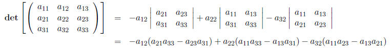
For example, we can write the determinant of a general 3×3 matrix by expanding along the second
column:

Note that all three definitions of the determinant are equivalent, and thus will give the same result.

3.2 Properties

Definition 25 A square matrix is called upper triangular is all of the matrix elements below the
diagonal are zero, and lower triangular is all of the matrix elements above the diagonal are zero.

Remark 12 The determinant of a triangular (upper or lower) matrix is equal to the product of
the diagonal elements.

Theorem 8 If A and B are n × n matrices, then det(AB) = det(A)det(B).

Remark 13 Combining these two results, we have

Remark 14 det(A^T) = det(A).

3.3 Computing the matrix inverse

Recall the definition above for the submatrix A_ij obtained from the matrix A by deleting the ith
row and jth column.

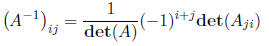
Theorem 9 If A is a n × n matrix and det(A) ≠ 0, then matrix elements of A^-1 are:

Thus, the determinant provides a way to tell if a matrix is invertible or not.

Corollary 10 A n × n matrix A is invertible if and only if det(A) ≠ 0.

For example, the inverse of a 2 × 2 matrix

can be computed by

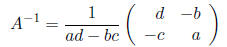
as long as ad − bc ≠ 0.

4 Complex numbers

4.1 Properties

Definition 26 A complex number z is a number of the form z = x + iy where x, y ∈R and
The real part of a complex number z = x + iy is x, and the imaginarypart is y. Note
that i^2 = −1.

Two complex numbers are said to be equal, a + ib = c + id, if and only if a = c and b = d.

We add two complex numbers by their real and imaginary parts respectively:

(a + ib) + (c + id) = (a + c) + i(b + d)

Multiplication of two complex numbers a+ib and c+id is performed by multiplying the binomials:

Definition 27 The complex conjugate of a complex number z = x + iy is

Definition 28 The absolute value of a complex number z = x + iy is

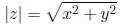
Note that

We can divide two complex numbers (a+ib) and (c+id) by using the complex conjugate as follows:

4.2 Polar coordinates

Complex numbers can be though of as as points in the xy-plane with the x-coordinate being the
real part, and the y-coordinate being the imaginary part. We can also represent points in the plane
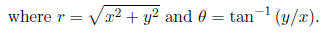
in polar coordinates using a length r and angle θ where x = r cosθ and y = r sinθ . Thus, we can
write a complex number as

Definition 29 The exponential of a complex number is defined as

This allows us to write any complex number in a polar form using the exponential function:

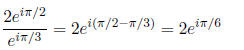
Multiplication and division of complex numbers written in exponential form then becomes simply
a matter of using the exponential properties of adding and subtracting exponents, respectively. For
example, we can compute

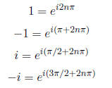
Note that the following complex exponential representations of the numbers 1,−1, i,−i, for any
integer n:

The exponential representation can be useful for finding complex roots of polynomials. For example,
consider finding the roots of n and solve the equation

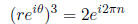
which results in the two equations:

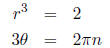
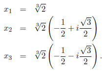
where n is an integer. Since we have a polynomial of degree 3, we are looking for 3 complex roots
so we consider n = 0, 1, 2. This gives us 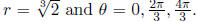The three roots of x^3 − 2 = 0
are then:

5 Eigenvalues and Eigenvectors

5.1 Eigenvalues

Definition 30 An eigenvalue of the n × n matrix A is a scalar λ such that

for some n × 1 column vector x.

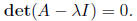
Alternatively, an eigenvalue is a scalar λ such that the equation

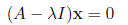
has a nonzero solution x. In order for this equation to have a nonzero solution, the matrix A − λI
must not be invertible, thus

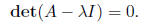
Computing this determinant for the matrix A−λI yields a polynomial in which in general admits
complex roots.

Definition 31 The characteristic polynomial of a matrix A is the polynomial in λ obtained
from computing the determinant

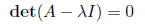
For example, if A is a 2 × 2 matrix

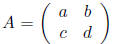
we can find the eigenvalues of A by computing det(A − λI) = 0 which gives us the characteristic
polynomial

which can be solved using the quadratic formula.

5.2 Eigenvectors

Definition 32 An eigenvector x associated with an eigenvalue λ is a nonzero solution to the
equation

Finding eigenvectors for a particular eigenvalue λ is then equivalent to finding the kernel of the
matrix (A − λI).

5.3 Examples

Consider the matrix

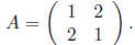
First, compute the eigenvalues by solving

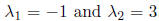
to get

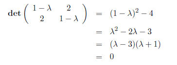
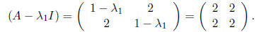
and thus the eigenvalues are . To find the eigenvector associated with ,
compute the kernel of the matrix

We want to find numbers such that

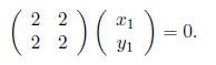
This results in the the equation 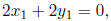which has a solution anytime that

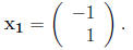
We can express this solution as

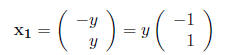
or simply as any scalar multiple of

Similarly, for the second eigenvalue we want to find numbers such that

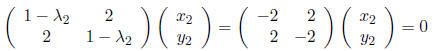
which gives us the solution , and thus any scalar multple of

or simply

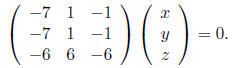
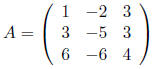
Now, let’s consider the 3 × 3 matrix

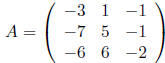
and find its eigenvalues and eigenvectors. By computing the determinant det(A − λI) we obtain
(after some work) the characteristic polynomial of A

which has roots Thus, there are only two unique eigenvalues
because −2 is repeated.

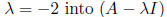
To find the eigenvector associated with , we find the kernel of the matrix by finding
(x, y, z) such that

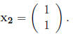
This yields the equations x = 0 and y = z, so the eigenvector associated with the eigenvalue λ = 4
is any scalar multiple of

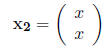
Plugging the other eigenvalue and solving for the eigenvector gives us

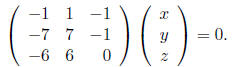
This gives us the equations z = 0 and x = y, so the eigenvector is any scalar multiple of

but this leaves us with only two eigenvectors for a 3 × 3 matrix. The last eigenvector in this case
is then the trivial vector

5.4 Determinants and eigenvalues

If you have the eigenvalues of a matrix, then you know its determinant by simply multiplying the
eigenvalues together.

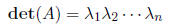
Theorem 11 If A is a n×n matrix, and are the eigenvalues of A (counting multiple
eigenvalues), then

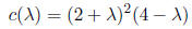
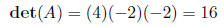
For example, consider the matrix

which has the characteristic polynomial 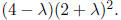Then, using the theorem

6 The Big Theorem

Now, we tie together all of the previous sections into one big theorem. This is very important

Theorem 12 If A is an n × n matrix, then the following are equivalent:

1. A is invertible
2. det(A) ≠ 0
3. kernel(A) = 0
4. has a unique solution
5. the rows of A are linearly independent
6. the columns of A are linearly indepdent
7. all of the eigenvalues of A are nonzero

What this means is that all of these conditions are equivalent: if you know condition is true, then
they all are true; or if one condition is false, then they all are false.